Measurement Model
Overview
It is possible to choose among various measurement models for a given EKF implementation. A particular model is selected based on many factors, one being the limitations of the available measurements. This formulation being described was selected due to the incomplete knowledge of the magnetic environment of the system and uses the available sensor information as follows:
#. Accelerometers “level” the system (used to compute \({^{\perp}}{\phi}{_{meas}^{B}}\) and \({^{\perp}}{\theta}{_{meas}^{B}}\)) FN
#. Magnetometers and/or GPS heading information align the \(\perp\)-frame with true or magnetic north (\({^{N}}{\psi}{^{\perp}}\))
#. GPS position and velocity measurements update the position and velocity estimates (\(\vec{r}^{N}\) and \(\vec{v}^{N}\))
Based upon these steps, the measurement vector, \(\vec{z}_{k}\), is formed:
\[\vec{z}_{k} = { \begin{Bmatrix} { \begin{array}{c} {\vec{r}_{GPS}^{N}} \cr {\vec{v}_{GPS}^{N}} \cr {^{N}}{\vec{\Theta}}{_{meas}^{B}} \end{array} } \end{Bmatrix} }\]with the corresponding measurement model, \(\vec{h}_{k}\):
\[\vec{h}_{k} = { \begin{Bmatrix} { \begin{array}{c} {\vec{r}_{pred}^{N}} \cr {\vec{v}_{pred}^{N}} \cr {^{N}}{\vec{\Theta}}{_{pred}^{B}} \end{array} } \end{Bmatrix} }\]Both \({^{N}}{\vec{\Theta}}{_{meas}^{B}}\) and \({^{N}}{\vec{\Theta}}{_{pred}^{B}}\) are 3x1 column vectors containing the roll, pitch, and heading values.
Measurement Model
The measurement model, \({\vec{h}_{k}}\) relates the system states, \({\vec{x}_k}\), to the system measurements. The position and velocity elements of this vector come directly from the position and velocity states, while \({^{N}}{\Theta}{_{pred}^{B}}\) is computed from \({^N}\vec{q}_{pred}^{B}\), as follows:
\[\begin{split}{^{\perp}{\phi}_{pred}^{B}} &= atan2 \begin{bmatrix} {2 \cdot \begin{pmatrix} {q_{2} \cdot q_{3}+q_{0} \cdot q_{1}} \end{pmatrix},{q_{0}}^{2}-{q_{1}}^{2}-{q_{2}}^{2}+{q_{3}}^{2} } \end{bmatrix}\\ {\hspace{5mm}} \\ {^{\perp}{\theta}_{pred}^{B}} &= -asin \begin{bmatrix} {2 \cdot \begin{pmatrix} {q_{1} \cdot q_{3}-q_{0} \cdot q_{2}} \end{pmatrix} } \end{bmatrix}\\ {\hspace{5mm}} \\ {^{N}{\psi}_{pred}^{\perp}} &= atan2 \begin{bmatrix} {2 \cdot \begin{pmatrix} {q_{1} \cdot q_{2}+q_{0} \cdot q_{3}} \end{pmatrix},{q_{0}}^{2}+{q_{1}}^{2}-{q_{2}}^{2}-{q_{3}}^{2} } \end{bmatrix}\end{split}\]
Measurement Vector (:math:`vec{z}_{k}`)
The measurement vector, \(\vec{z}_{k}\) is comprised of position, velocity, and attitude information as defined above. It is formed from sensor measurements. However, only the GPS velocity is directly available from measurements; other information must be derived from sensor readings using the relationships described below.
Roll and Pitch Measurements
Roll and pitch values are computed from the accelerometer signal. Under static conditions, measurements made by the accelerometer consists solely of gravity and sensor noise. Along the axis pointed in the direction of gravity, the sensor measures -1 [g]. This is due to the proof-mass being pulled in the direction of gravity, which, in the absence of gravity, is equivalent to a deceleration of 1 [g].
\[\vec{a}_{meas} = \vec{a}_{grav} = -\vec{g}\]Static roll and pitch values are determined by noting that gravity is constant in the N-Frame (perp-Frame):
\[\begin{split}\vec{g}^{N} = \vec{g}^{\perp} = \begin{Bmatrix} \begin{array}{c} 0 \\ 0 \\ 1 \end{array} \end{Bmatrix}\end{split}\]and can be transformed into the body frame through \({^{B}{R}^{\perp}}\):
\[\begin{split}\vec{g}^{B} = {^{B}{R}^{\perp}} \cdot \vec{g}^{\perp} = { \begin{pmatrix} { {^{\perp}{R}^{B}} } \end{pmatrix} }^{T} \cdot \vec{g}^{\perp} = { \begin{pmatrix} { {^{\perp}{R}^{B}} } \end{pmatrix} }^{T} \cdot \begin{Bmatrix} \begin{array}{c} 0 \\ 0 \\ 1 \end{array} \end{Bmatrix}\end{split}\]Using the definition of \({^{\perp}{R}^{B}}\) (discussed in Attitude Parameters) and expanding the equation, the accelerometer measurements can be related to roll and pitch angles:
\[\vec{g}^{B} = -\vec{a}_{meas}^{B}\]\[\begin{split}\begin{Bmatrix} { \begin{array}{c} {-sin \begin{pmatrix} { {^{\perp}{\theta}^{B}} } \end{pmatrix}} \cr {cos \begin{pmatrix} { {^{\perp}{\theta}^{B}} } \end{pmatrix} \cdot sin \begin{pmatrix} { {^{\perp}{\phi}^{B}} } \end{pmatrix}} \cr {cos \begin{pmatrix} { {^{\perp}{\theta}^{B}} } \end{pmatrix} \cdot cos \begin{pmatrix} { {^{\perp}{\phi}^{B}} } \end{pmatrix}} \end{array} } \end{Bmatrix} = { \begin{Bmatrix} { \begin{array}{c} {-a}_{mx}^{B} \\ {-a}_{my}^{B} \\ {-a}_{mz}^B \end{array} } \end{Bmatrix} }\end{split}\]From this result, the angles corresponding to the accelerometer signal are found:
\[{^{\perp}}{\phi}{_{meas}^{B}} =atan2(-a_{my}^{B},-a_{mz}^{B} )\]\[{^{\perp}}{\theta}{_{meas}^{B}} =-asin(-\hat{a}_{mx}^{B} )\]where, \(\hat{a}_{mx}^{B}\) is the x-axis acceleration value normalized by the total acceleration magnitude:
\[\hat{a}_{mx}^{B} = { {a_{mx}^B} \over \| {\vec{a}_{meas}^{B}} \|}\]Normalization of the y and z-axis accelerometer values can be performed. However this is not required as the \(atan\) function uses the ratio of the two (the normalization factor cancels out).
Heading Measurements
Heading measurements are determined from one (or both) of the following:
- Magnetometers
- GPS Velocity
Magnetometer-Based Heading
Magnetometers measure the local magnetic field at a high DRs but the readings can be affected by hard and soft-iron disturbances in the system or by changes in the external magnetic field. Hard and soft-iron effects are local to the system and can be accounted for; external field disturbances cannot be corrected.
Adjustment of the magnetic field measurement for hard/soft-iron disturbances can be performed according to the following equation:
\[\vec{m}_{corr}^{B} = R_{SI} \cdot S_{SI} \cdot {R_{SI}}^{T} \cdot (\vec{m}_{meas}^{B} - \vec{m}_{bias}^{B} - \vec{m}_{HI}^{B} )\]where \(\vec{m}_{meas}^{B}\) is the measured magnetic field vector in the body-frame, \(\vec{m}_{HI}^{B}\) is the hard-iron disturbance, and \(R_{SI}\) and \(S_{SI}\) are the soft-iron disturbances.
Note
For this analysis the magnetometer bias is neglected; assumed to be negligible or lumped in with the hard-iron.
Hard and soft-iron parameters are estimated by performing a magnetic-alignment maneuver.
Note
The application of these corrections do not adjust individual magnetometer channels to match the actual field strength. Only the relative magnetic field is corrected, resulting in a unit-circle for the xy magnetic-field. However, as shown later, this enables the heading to be calculated from the corrected signal.
Heading calculation
The heading is computed using the fact that, in the magnetic NED-frame, the y-axis component of the magnetic field is zero. In the true-north NED-frame this is not the case; a magnetic declination angle corrects for this. The magnetic field at a given point can be found using the World Magnetic Model (WMM) or from NOAA’s website (https://www.ngdc.noaa.gov/geomag-web/#igrfwmm). In San Jose, CA, the magnetic field estimates are provided in Table:
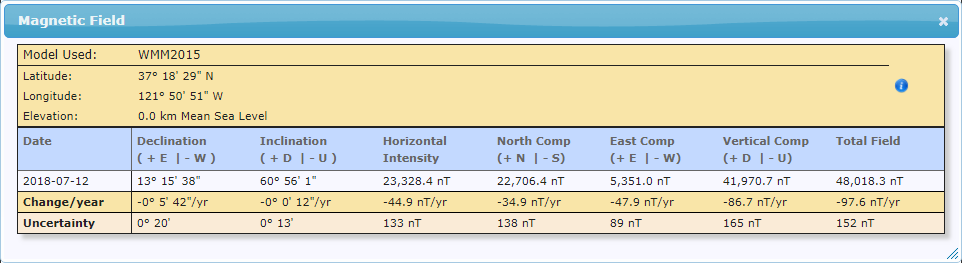
Magnetic Field Components based on WMM
Figure illustrates the relationship between the Lines of constant Lat/Lon, the NED-frame, and the perp-frame. Declination is specified with \(\delta\) and heading is specified with \(\psi\).
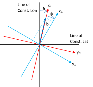
Relationship of Magnetic-Field to N and B-Frames
The magnetic field vector, \(\vec{b}\), can be broken down into two components:
- the xy-plane component and
- the vertical component
The relationship between heading and magnetic field is based on the components of \(\vec{b}^{N}\) as measured in the NED-frame:
\[\begin{split}\vec{b}^{\perp} = {^{\perp}{R}^{N}} \cdot \vec{b}^{N} = {^{\perp}{R}^{N}} \cdot \begin{Bmatrix} \begin{array}{c} b_{xy} \\ 0 \\ b_{z} \end{array} \end{Bmatrix}\end{split}\]Expanding the expression results in the following:
\[\begin{split}\begin{Bmatrix} \begin{array}{c} b_{x}^{\perp} \\ b_{y}^{\perp} \\ b_{z}^{\perp} \end{array} \end{Bmatrix} = \begin{Bmatrix} \begin{array}{c} b_{xy} \cdot cos{ \begin{pmatrix} { {^{N}{\psi}^{\perp}} } \end{pmatrix} } \\ -b_{xy} \cdot sin{ \begin{pmatrix} { {^{N}{\psi}^{\perp}} } \end{pmatrix} } \\ b_{z}^{\perp} \end{array} \end{Bmatrix}\end{split}\]From this, the heading is computed:
\[tan{ \begin{pmatrix} { {^{N}{\psi}^{\perp}} } \end{pmatrix} } = { {b_{xy} \cdot \sin{ \begin{pmatrix} { {^{N}{\psi}^{\perp}} } \end{pmatrix} }} \over {b_{xy} \cdot \cos{ \begin{pmatrix} { {^{N}{\psi}^{\perp}} } \end{pmatrix} }} } = { {-b_{y}^{\perp}} \over {b_{x}^{\perp}} } = { {-m_{corr,y}^{\perp}} \over {m_{corr,x}^{\perp}} }\]Note
The values for \(b_{x}^{\perp}\) and \(b_{y}^{\perp}\) are the corrected and ‘leveled’ values of the measured magnetic-field in the body-frame; roll and pitch estimates are used to level the signal via \({^{\perp}{R}_{pred}^{B}}\).
\[{\vec{m}_{corr}^{\perp}} = {^{\perp}{R}_{pred}^{B}} \cdot {\vec{m}_{corr}^{B}}\]Note
As this calculation only corrects the magnetic-field in the xy body-frame, the heading solution is best when the system is nearly level. he solution begins to degrade as the roll and pitch increase. This can be accounted for by adjusting the measurement covariance matrix, \(R\), accordingly. Additionally, the solution also begins to degrade as the iron in the system increases.
GPS Heading
Heading is also provided directly from the GPS messages. The four messages currently decoded by the IMU381/OpenIMU firmware provide true heading via messages listed in Table.
GPS Messaging and Heading Measurement¶ System Message Description Units NovAtel BESTVEL [deg] NMEA VTG True track made good [deg] SiRF [deg x 100] ublox NAV-VELNED Heading of motion 2-D [deg]
Choosing the Heading Measurement Source
Deciding upon the source of the heading information is ultimately up to the user. In the Aceinna algorithm, the source switches from GPS to magnetometer based on the operating condition. Specifically, during periods of motion, GPS measurements are used as the are considered more accurate as they are not influenced by the magnetic environment. However, when at rest the GPS heading provides no heading information. In this case, the magnetometer provides heading information.
This implementation requires the algorithm to switch not only the source of the data but also the related measurement covariance values.
GPS Position and Velocity
GPS-based position is derived from the GPS lat/lon/alt message (BestPos, GGA, etc) and converted to NED-position using the WGS84 model.
GPS-based velocity is obtained from the BestVel, etc message. However, the NMEA message does not provide vertical velocity, derived from or accounted for in other ways. In all cases the N and E-velocity is calculated from heading and ground speed. The relationship is: